
Excel SUMIF Function
Excel SUMIF function returns the sum of a range of cells based on a single criteria or condition.
- Fundamentals of SUMIF function.
- Anatomy of SUMIF Syntax.
- SUMIF function with Numeric Conditions (greater than, less than, equal).
- SUMIF with text criteria
- SUMIF with Date Condition
- SUMIF with Wildcard
- SUMIF with Named Range
- Add two or more SUMIF formulas
- SUMIF with AND/OR condition
- Common Problems and answers on SUMIF function.
1. Fundamentals of SUMIF function
Excel users use SUMIF function to sum the values in a range based on a single criteria specified by the users. The criteria or condition may be based on numbers, text, and dates. Microsoft categorizes the function under Math and Trigonometry Functions. SUMIF function supports both logical operators (>, <, <>, =, <=, >=) and Wildcard (*, ?). Before going to solve real world problems, let’s see some basic information on SUMNIF:
- SUMIF adds values in a range based on single criteria.
- Criteria may be based on numbers, text, and dates.
- SUMIF function supports both logical operators (>,<, <>, =, <=, >=) and Wildcard (*,?).
- The criteria of text strings argument can be a maximum of 255 character long. Longer than 255 characters will return a #VALUE! error.
- SUMIF function returns incorrect results when the range in the first argument is not in the same shape and size in the second argument.
- Users can add two or more SUMIF formula as =SUMIF(Range_Criteria, SUM Range)1+SUMIF(Range_Criteria, SUM_Range)2+SUMIF(Range Criteria, SUM Range)n
2. Anatomy of SUMIF Syntax
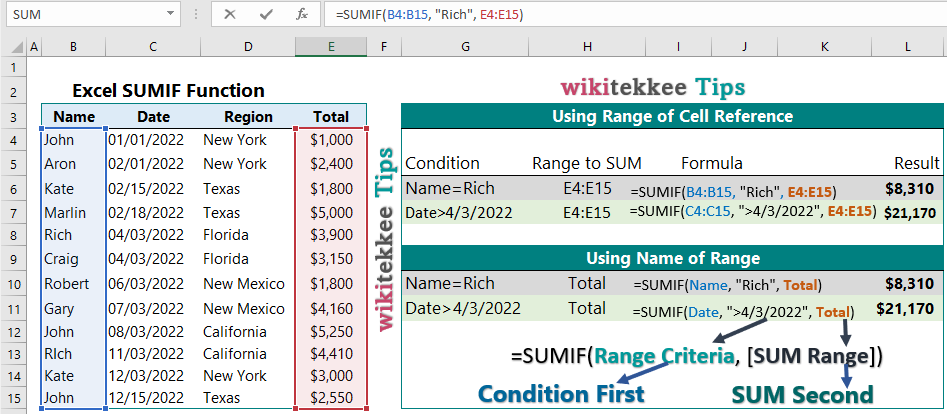
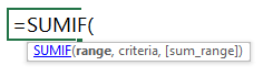
The base formula of SUMIF is =SUMIF(range, criteria, [sum_range]). Let’s explain the different parts of the formula:
Part 1: Range and criteria of the cells on which the first condition is used. For example, SUMIF the Name of the employee is Rich. Then, we write =SUMIF(Name, “Rich”,. The criteria is the REQUIRED part of the SUMIF function syntax.
Part 2: Sum_range is the range of cells from which we want to add values. For Example, we want to add total for Rich. The SUM range is an optional part. However, if the SUM range part is excluded from the syntax, Excel will add the cells specified in the range argument.
Be Careful! Any text, logical, or mathematical criteria MUST be enclosed in double quotation marks (” “). If the criteria is numeric, the double quotation marks are NOT required.

Quick tips from wikitekkee.com:
In the SUMIF formula, the criteria range comes first, and then Excel takes the SUM range. We have been teaching our clients and students one quick tip. Just read the formula like IF+SUM, where the condition (IF) comes first, and then SUM. We have visualized the SUMIF formula as IF + SUM as follows.

3. SUMIF Function with Numeric Condition
Example 1: Numeric Condition (greater than “>”)
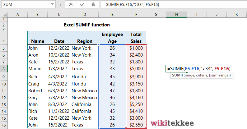
Question: What is the total sales of the employees who are more than 33 years old?
Answer: =SUMIF(E5:E16, “>33”, F5:F16), which returns the value of $19,820.
Example 2: Numeric Condition (Less than, “<“)
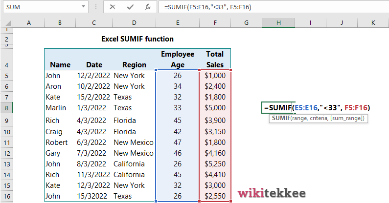
Question: What is the total sales of the employees who are less than 33 years old?
Answer: The formula =SUMIF(E5:E16,”<33″, F5:F16), which returns the value of $13,600.
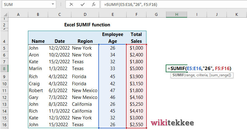
Example 3: Numeric Condition (equal to “=”)
Question: What is the total sales of employees who are exactly 26 years old?
Answer: The formula =SUMIF(E5:E16,”26″, F5:F16), which returns the value of $8,800.
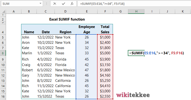
Example 4: Numeric Condition (greater than or equal to “>=”)
Question: What is the total sales of the employees whose age are more than or equal to 34 years old?
Answer: The formula =SUMIF(E5:E16,”>=34″, F5:F16), which returns the value of $19,820.
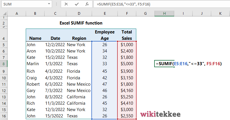
Example 5: Numeric Condition (less than or equal to “>=”)
Question: What is the total sales of employees whose age are less than or equal to 33 years old?
Answer: The formula =SUMIF(E5:E16,”<=33″, F5:F16)
4. SUMIF with text criteria
Users can use SUMIF function with text criteria. The syntax of the SUMIF function with text criteria is as follows:
=SUMIF(criteria_range, “text_criteria”, [sum_range])
Where,
- criteria_range is the range of cells containing the text criteria.
- “text_criteria” is the text criteria included within the double quotation (” “).
- sum_range is the range of cells from which the values will be added.
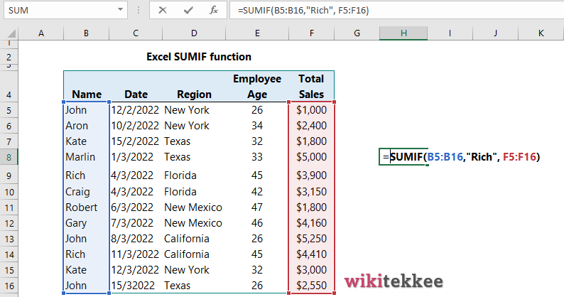
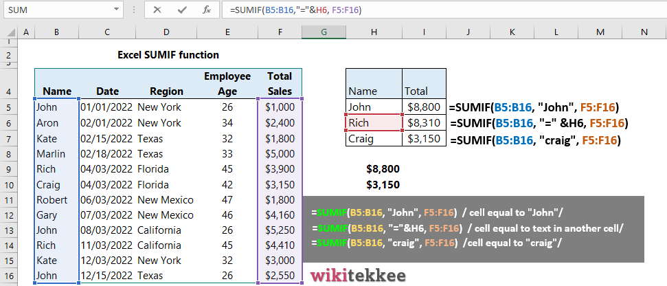
Example 6: SUMIF function with text criteria (cell reference is equal to specific text)
Question: What is the total sales of the employee Rich?
Answer: The formula =SUMIF(B5:B16,”Rich”, F5:F16), which returns the value of $8,310.
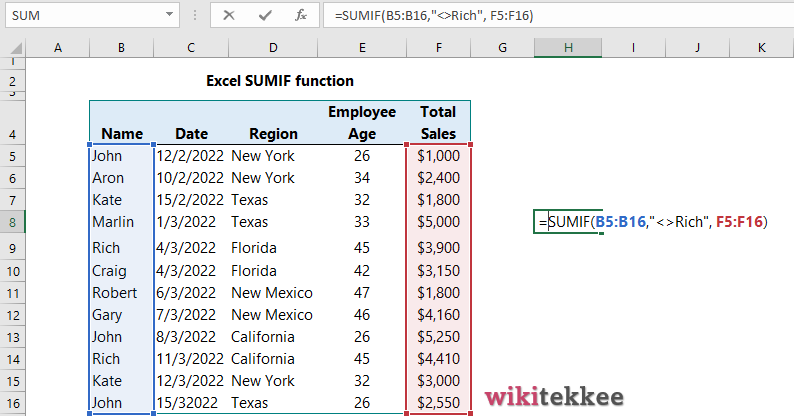
Example 7: SUMIF function with text criteria (cell reference is not equal to specific text)
Question: What is the total sales when employee is NOT Rich?
Answer: The formula =SUMIF(B5:B16,”<>Rich”, F5:F16), which returns the value of $30,110.
Example 8: SUMIF with text criteria (text reference is from another cell)
Question: What is the total sales when employee name is equal to H6?
Answer: The formula =SUMIF(B5:B16, “=” &H6, F5:F16), which returns the value of $8,310.
5. SUMIF with date Condition
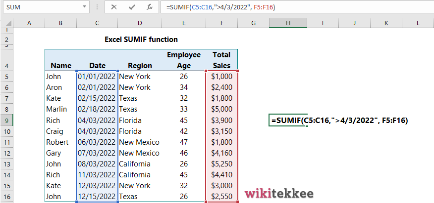
Example 9: SUMIF with date criteria (cell reference is after a specific date)
Question: What is the total sales after April 3, 2022?
Answer: The formula =SUMIF(C5:C16,”>4/3/2022″, F5:F16), which returns the value of $21,170.
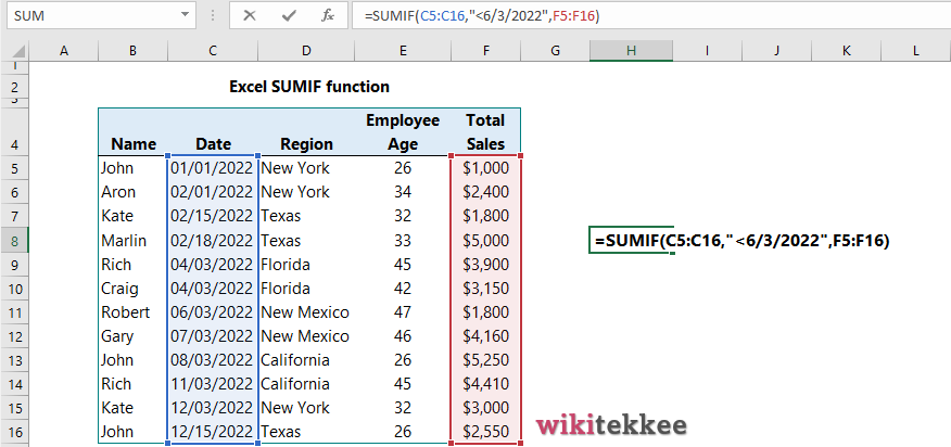
Example 10: SUMIF with date criteria (cell reference is before a specific date)
Question: What is the total sales before June 3, 2022?
Answer: The formula =SUMIF(C5:C16,”<6/3/2022″,F5:F16), which returns the value of $17,250.
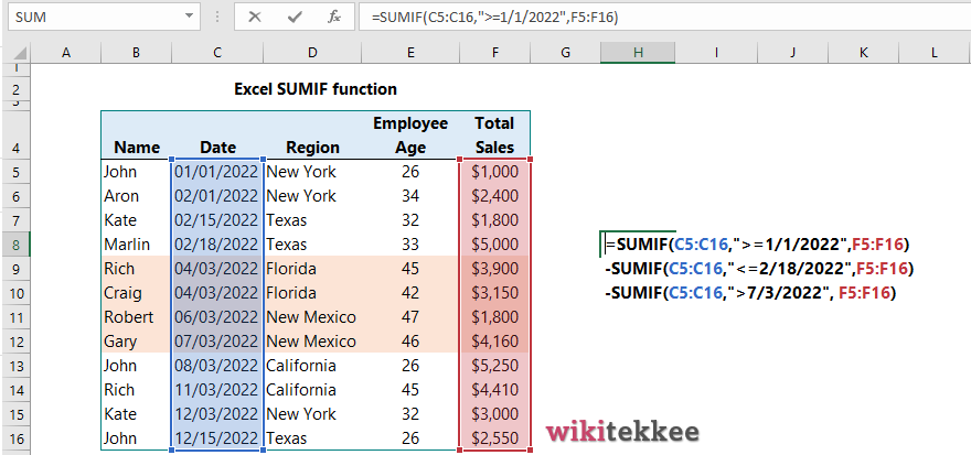
Example 11: SUMIF between two dates
Question: What is the total sales between March and July, both dates inclusive?
Answer: The formula =SUMIF(C5:C16,”>=1/1/2022″,F5:F16) -SUMIF(C5:C16,”<=2/18/2022″,F5:F16) -SUMIF(C5:C16,”>7/3/2022″, F5:F16), which returns the value of $13,010.
6. SUMIF with Wildcard (*,?,~)
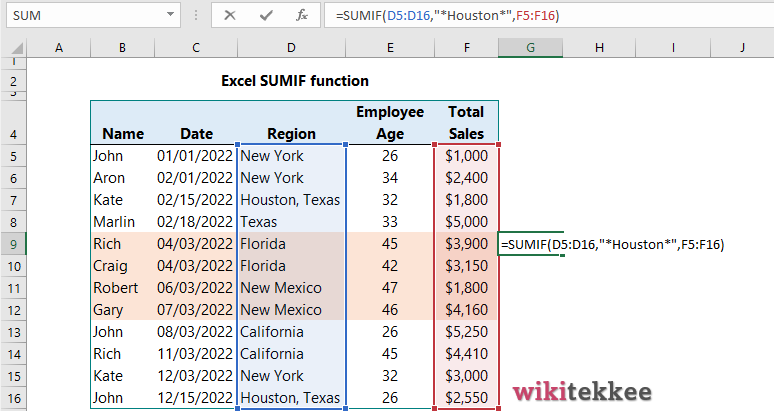
Example 12: SUMIF with Asterisk (*) wildcard:
Question: What is the total sales of Houston?
Answer: The formula =SUMIF(D5:D16,”Houston“,F5:F16), which returns the value of $4,350.
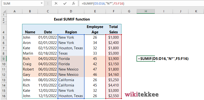
Example 13: SUMIF with text at the start (wildcard)
Question: What is the total sales of the state names starting with N?
Answer: The formula =SUMIF(D5:D16,”N*”,F5:F16), which returns the value of $12,360.
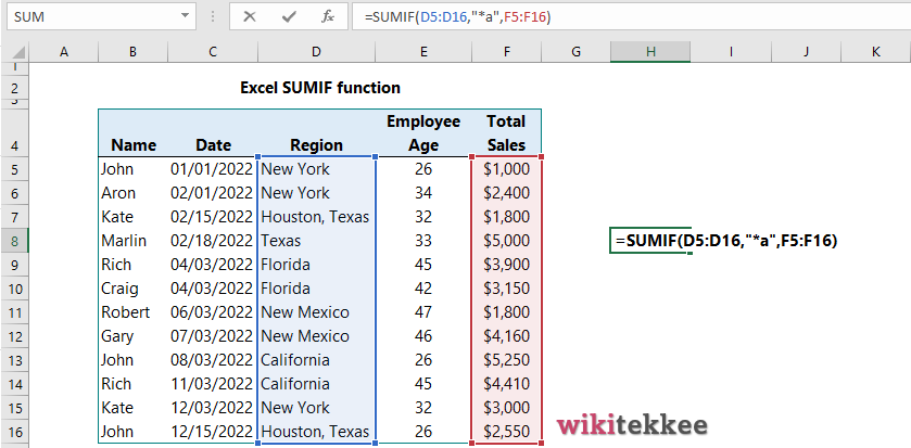
Example 14: SUMIF with text at the end (wildcard)
Question: What is the total sales of the states that end with a?
Answer: The formula =SUMIF(D5:D16,”*a”,F5:F16), which returns the value of $16,710.
7. SUMIF with Named Range
Instead of using the cell references, users can use the named range. In our example, we have named the ranges as follows:
B5:B16 =Name
C5:C16 =Date
F5:F16 = Total
Now, instead of using the cell reference B5:B16, we can use Name.
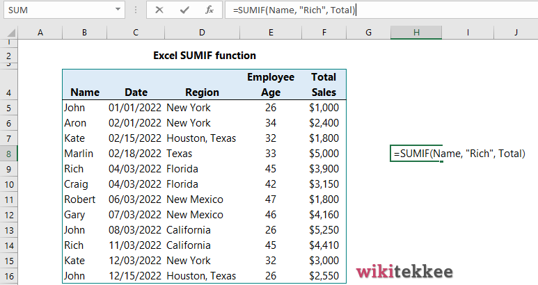
Example 15: SUMIF with Named Range
Question: What is the total sales of Rich?
Answer: The formula with Named Range: =SUMIF(Name, “Rich”, Total), which returns the value of $8,310.
8. How to add two or more SUMIF formulas
Sometimes, users need to add two or more SUMIF formulas. It helps to add more conditions. Let’s take an example.
Example 16: Adding two SUMIF formulas for multiple conditions.
Question: What is the total sales of Rich and John?
Answer: The formula: =SUMIF(B5:B16, “Rich”, E5:E16)+ SUMIF(B5:B16, “John”, E5:E16), which returns the value of $17,110.

9. SUMIF with AND/OR condition
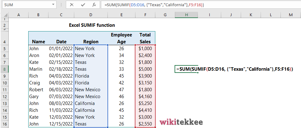
We want to know the total sales from the regions Texas OR California.
Example 17: SUMIF with OR condition.
Question: What is the total sales from the regions Texas or California?
Answer: The formula: =SUM(SUMIF(D5:D16, {“Texas”,”California”},F5:F16)), which returns the value of $19,010.
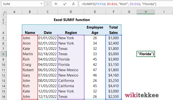
Example 18: SUMIFS with AND Condition:
To use the AND condition, it is better to use SUMIFS (with s).
Example 18: SUMIFS with AND condition.
Question: What is the total sales of Rich and Florida?
Answer: The formula: =SUMIFS(F5:F16, B5:B16, “Rich”, D5:D16, “Florida”), which returns the value of $3,900.
10. Common Problems and Answers on SUMIF function:
Problem 1: Why my SUMIF function returns incorrect values?
Answer: SUMIF function returns incorrect results when the range in the first argument is not in the same shape and size in the second argument.
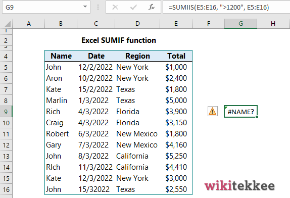
Problem 2: Why am I getting the #NAME! error message?
Answer: The #NAME! error indicates that something in your formula needs to be corrected. For example, in the image below, we have intentionally mistyped the formula as SUMIIS (see two i’s and S instead of F) instead of SUMIF. It means that we have mistyped the formula and are getting the error #NAME! message. One suggestion from Microsoft is NOT to use error-handling function such as IFERROR to mask the error.
This is a very good tips especially to those new to blogosphere, brief and accurate information… Thanks for sharing this one. A must read article.