
Correlation in Excel with P-Value
The Correlation in Excel with P-value can be calculated in two different ways. The first method is to calculate the P-value by using formula, and the second one is to use regression analysis, which automatically produces the p-value. In this section, we will discuss both the methods.
In this section:
- What is P-Value in correlation?
- How to Calculate P-Value using Excel formula?
- How to calculate P-Value of Correlation using regression analysis.
- More related readings.

1. What is p-value?
The P-value tells us whether the relationship between two variables are statistically significant. In order to determine whether the correlation between two variables, meaning the change in one variable with the changes in another variable, is statistically significant, we need to calculate t-score or p-value. In practically research, both the t-score and p-value are commonly used. We discuss how calculate both t-score and p-value.
2. How to Calculate P-Value using Excel formula:
To calculate P-Value by using the TDIST Excel Function, follow the steps below:
Step 1: Calculate the Pearson Correlation between two variables:
To calculate the Pearson Correlation between two variables, the formula we use in our example is =PEARSON(C6:C15,D6:D15)
Step 2: Calculate the number of observations:
In our example, the total number of observations (N) is 10.
Step 3: Calculate T-statistics:
The formula to calculate the T-statistics is =J5*(SQRT(J7-2))/SQRT(1-J5^2)


Step 4: Calculate Degree of Freedom:
The degree of freedom is =N-2, which is 8 in our example.
Step 5: Calculate P-value:
To calculate the P-value, the formula is =TDIST(J9,J11,2), which returns the P-value of 0.000002, indicating that the correlation between hours study and grade point average (GPA) is highly significant.
3. Calculate P-Value using Regression Analysis:
To calculate P-value using regression analysis, follow the steps below:
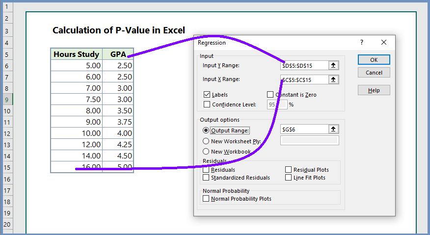
Step 1: Click Data (as in 1)–> then click Data Analysis (as in 2)–> Click Regression (as in 3)–> Then click OK.

Step 2: After clicking OK in step 1, you will see the regression dialogue box as in the image below. Now, you should select the Y-range (Dependent variable) and the X-range (Independent variable). In our example, we have selected D5:D15 as our Y-range, and C5:C15 as our X-range. We have selected with the names of the variables; therefore, checked Labels. We have also selected output range, in which cell the regression output will be generated. Finally click OK.
Step 3: Finally, we have edited the regression summary and present the results as follows:
From the table below, we can see both the T-statistics and p-value, and find that both them indicate that the correlation between hours study and GPA is highly significant.

More related readings:
- Correlation in Excel Data Analysis
- Excel CORREL Function
- Excel CORREL Function MS Office Post
- Multiple Correlation in Excel Analysis Tool Pack
- Multiple Regression in Excel
- Predict a Variable based on other Variables in Excel Regression
I was very pleased to uncover this great site. I need to to thank you for ones time due to this fantastic read!! I definitely enjoyed every bit of it and I have you book-marked to see new things in your website.
Someone necessarily assist to make severely articles I might state. This is the first time I frequented your website page and thus far? I surprised with the research you made to make this particular publish amazing. Excellent process!