Excel SORT Function ( 5 Examples)

Excel SORT Function

The Excel SORT function returns the contents of a range or an array in ascending or descending order. The returned array is the same shape as the provided array argument. 

In this section:

---

1. Syntax of Excel SORT Function
2. How to use Custom SORT in Excel?
3. SORT by values.
4. SORT by location.
5. SORT by city and State.
6. SORT States in Ascending and Sales in Descending Order.

---

Download Excel SORT Data

1. Syntax:

=SORT(array,[sort_index],[sort_order],[by_col])

where:

array: The range or array users want to SORT.

[sort_index]: This is an optional argument and indicates a number of the row or column to be sorted.

[sort_order]: This is also an optional argument and indicates the desired sort order. For example, 1 for ascending order and -1 for descending order.

[by_col]: A logical value indicating the desired sort direction; FALSE to sort by row (default), TRUE to sort by column.

Notes:

1. Where sort_index remains empty, Excel assumes the sort either by row1 or by column1.
2. SORT Function sorts data in an array. To SORT data in the grid, users need to use SORTBY Function.
3. An array may be the values in a row, or in a column, or a combination of both.
4. SORT function returns an array and will spill it’s final results of a formula.
5. Dynamic array does not work between workbooks.

Examples:

2. How to use Custom Sort in Excel:

To use the Excel built-in custom SORT, follow the steps below:

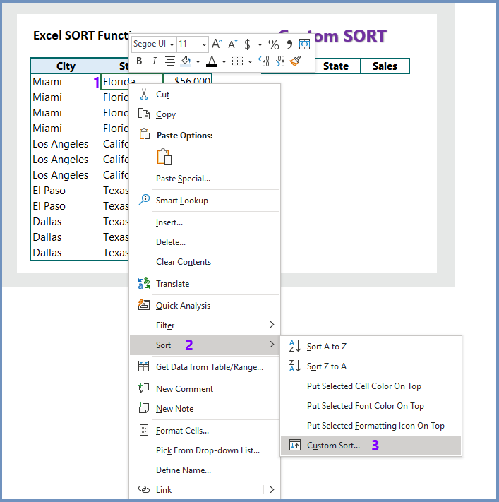
Step 1: Right-click on any cell (as 1 in image below).

Step 2: Click on Sort (2 as in image below).

Step 3: Click on Custom Sort (3 in image below)

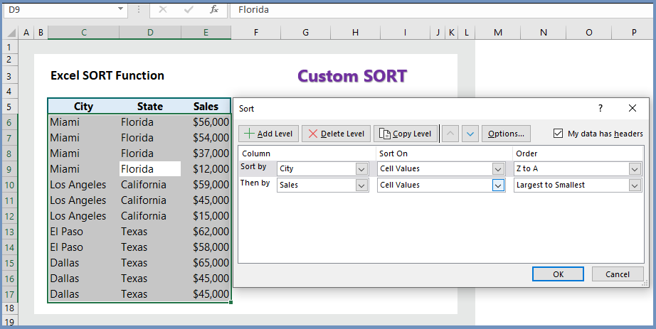
After clicking on Custom Sort, you will see the Sort dialogue box (as in the image below). Now you can define sort by variable, and then by, and then by. To add additional then by, click “Add Level“.

Example: Suppose, we want to SORT by city and sales and the sales will be sorted from Largest to Smallest. Then click OK.

3. SORT by values:

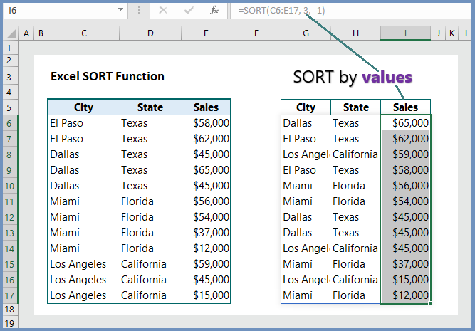
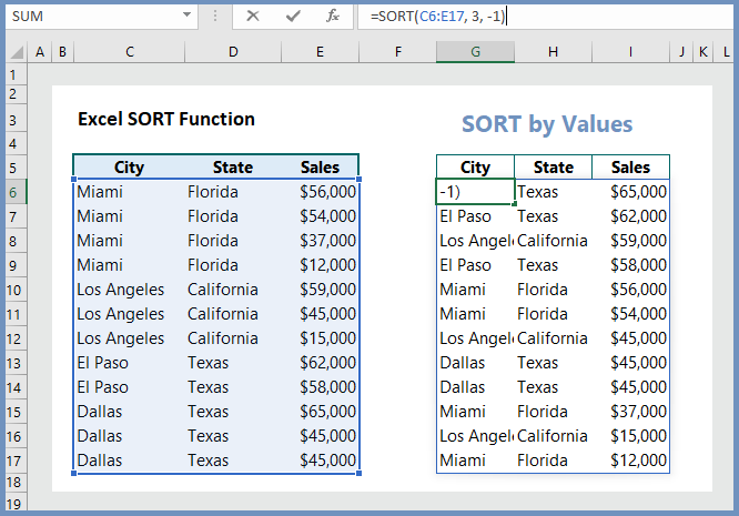
Suppose, we want to SORT by sales. The formula is =SORT(C6:C17, 3, -1), which sorts the data by sales. Remember that 3 is the column reference, and -1 indicates descending order.

4. SORT by location:

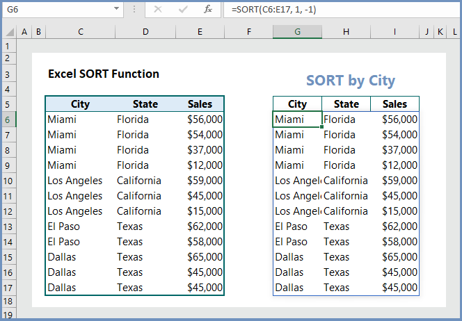
Suppose, we want to SORT by city the sales by descending order. The formula is =SORT(C6:C17, 1, -1), which sorts the data by city and sales. Remember that 1 is the column reference, and -1 indicates descending order.

5. SORT by city and State:

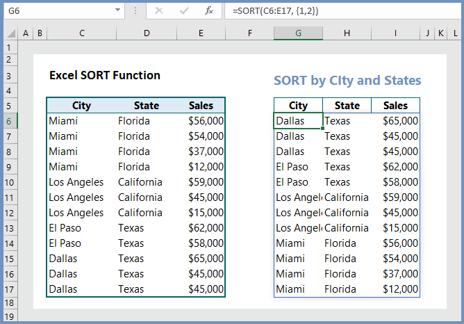
Suppose, we want to SORT by City and States. The formula is =SORT(C6:C17,{1,2}), which sorts the data by City and States. Remember that 1 and 2 are is the column references, and empty sort_order will sort the values by ascending order.

6. SORT States in Ascending and Sales in Descending Order:

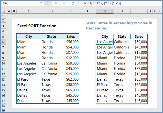
Suppose, we want to SORT by States in ascending and Sales revenues in descending order. The formula is =SORT(C6:C17,{2,3}, {1, -1}), which sorts the data by States in ascending and Sales revenue in descending order. Remember that the numbers {2, 3} within the first curly brackets are the column references and 1 and -1 indicate the order of sorting.

More related readings:

MS Office Post on SORT

Excel AVERAGE Function

Excel FILTER Function

Multiple Regression in Excel

Multiple Correlation in Excel

COUNTIF Function in Excel