
Excel MATCH Function
The Excel MATCH Function returns the location reference of a particular value in a cell or range or a table. The MATCH function can be used for partial matching, exact matching, and wildcards. The MATCH function is used combined with the INDEX Function.
In this section:
- Syntax
- Exact Match
- Approximate Match
- Wildcard Match
- Case-sensitive Match
- ISNA and MATCH
- INDEX/MACTH combination to find Names.

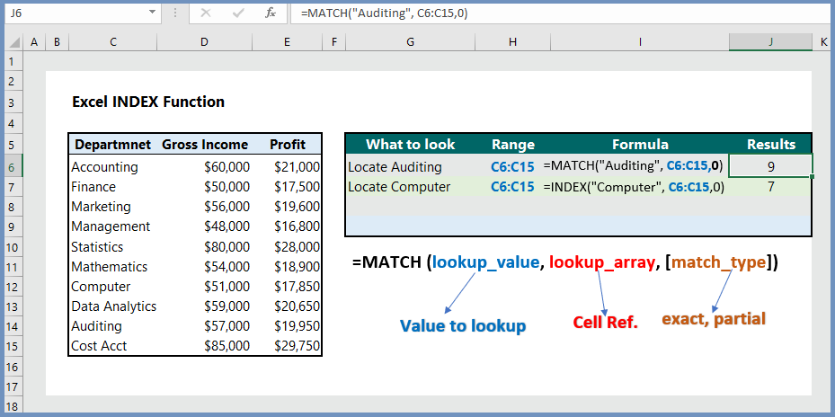
1. Syntax:
=MATCH (lookup_value, lookup_array, [match_type])
- lookup_value: The value for which users want to match with.
- lookup_array: Reference to a range of cells or an array reference.
- match_type: This is an optional argument, which indicates match type.
Match type:
- 0: Exact Match
- 1: Approximate Match
- -1: Approximate Match
Examples:
2. Return the Exact Match (0):
To return the Exact Match value, the formula is =MATCH(G5, C6:C14, 0), which returns the value of 6, the position of Milton in column C.

3. Return the Approximate Match (1):
To return the approximate match, the formula is =MATCH(G5, C6:C14, 1), which returns the value of 8, the approximate match with “Mi“.

4. Return value for Wildcard Match (?, *):
To return values for wildcard match, the formula is =MATCH(G5, C6:C14, 0), which returns the value of 6, the first match with “Mi”–Milton.

5. Return the case-sensitive Match ():
To return the value with case-sensitive match, the formula is {=MATCH(TRUE, EXACT(C6:C14, G5),0)}, which returns the value of 6, the position of lower case “rich“. We can check with the “Rich” (with upper case R) and will see the position is 2.

6. Return “Not in Dept A” if the values do not match:
The combination of ISNA and MATCH is used to compare the values in different cells. In our example, we wanted to check whether values in Dept A and Dept B are homogeneous. When Excel finds that the values are different from Dept B, it returns “Not in Dept A”, and the formula is =IF(ISNA(MATCH(D8, C:C, 0)), “Not in Dept A”, ” “).

7. INDEX/MATCH to find Names:
To find the names of person by department, we can use the INDEX/MATCH combination, and the formula is =INDEX(C6:C12, MATCH(H5, E6:E12, 0)).

More reading:
Yeah bookmaking this wasn’t a speculative conclusion great post! .
I truly appreciate this post. I’ve been looking everywhere for this! Thank goodness I found it on Bing. You’ve made my day! Thank you again
I am glad to be one of many visitants on this great website (:, regards for putting up.
whoah this blog is fantastic i love reading your articles. Keep up the great work! You know, lots of people are searching around for this info, you can help them greatly.
of course like your website but you have to check the spelling on quite a few of your posts. A number of them are rife with spelling issues and I in finding it very troublesome to tell the truth however I will definitely come again again.
I’ll immediately grab your rss feed as I can not in finding your email subscription hyperlink or e-newsletter service. Do you’ve any? Please permit me realize so that I may just subscribe. Thanks.
I like what you guys are up too. Such smart work and reporting! Keep up the excellent works guys I have incorporated you guys to my blogroll. I think it will improve the value of my web site 🙂
I am not rattling excellent with English but I find this real easy to translate.
An impressive share, I just given this onto a colleague who was doing a little analysis on this. And he in fact bought me breakfast because I found it for him.. smile. So let me reword that: Thnx for the treat! But yeah Thnkx for spending the time to discuss this, I feel strongly about it and love reading more on this topic. If possible, as you become expertise, would you mind updating your blog with more details? It is highly helpful for me. Big thumb up for this blog post!
We’re a group of volunteers and starting a new scheme in our community. Your website offered us with valuable information to work on. You’ve done a formidable job and our whole community will be thankful to you.
Thanks a lot for the blog.Thanks Again. Really Cool.
I always was interested in this subject and still am, appreciate it for posting.
Well I definitely liked studying it. This information provided by you is very effective for accurate planning.
obviously like your web-site but you have to check the spelling on quite a few of your posts. Many of them are rife with spelling problems and I find it very troublesome to tell the truth nevertheless I will surely come back again.
Today, while I was at work, my cousin stole my iPad and tested to see if it can survive a 30 foot drop, just so she can be a youtube sensation. My iPad is now broken and she has 83 views. I know this is completely off topic but I had to share it with someone!
All this, along with detailed click here profiles and tags so you know if a webcam model is right for you from the start.