Excel FILTER Function (5 Examples)

Excel FILTER Function

The Excel FILTER function allows users to filter a range of data based on criteria users define and returns matching values.

In this section:

---

1. Syntax of FILTER Function
2. FILTER the Sales revenue of certain location.
3. How to make the FILTER Dynamic.
4. #CALC! error and how to manage it.
5. FILTER values greater than a certain value.

---

Download the FILTER Data

1. Syntax

=FILTER (array, include, [if_empty])

where:

• array: The array, or range to filter.
• include: A Boolean array, which must have the same height or width as the array.
• [if_empty]: [optional] Value to return if all values included are empty.

Notes:

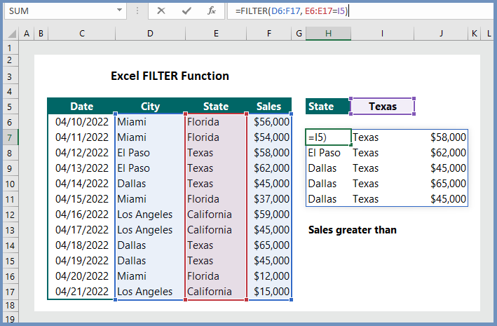
1. The defined array can be a row of values, a column of values, or a combination of rows and columns of values. In our example, the array to FILRER is the range D6:F17.
2. The Excel FILTER function will return an array, which will spill if it’s the final result of a formula, indicating that Excel will dynamically create the appropriate sized array range when you press ENTER.
3. Use the third argument as empty if the dataset has the potential of returning an empty value; otherwise, a #CALC! error will result, as the current version of Excel does not support empty arrays.
4. The Excel FILTER Function will return an error if any value of the include argument is an error (#N/A, #VALUE, etc.) or cannot be converted to a Boolean.

Examples:

2. Extract the sales revenue of the state of Texas:

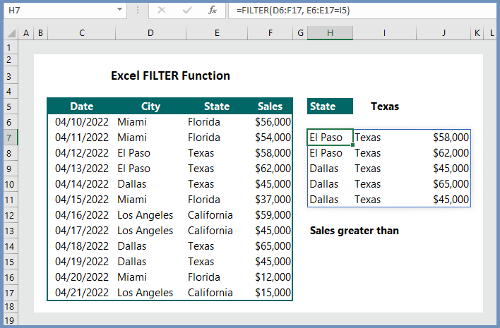
The extract the sales revenues of the state of Texas, we use the formula =FILTER(D6:F17, E6:E17=I5), which extract the sales revenues from Texas. We have use I5=Texas.

3. How can I create Dynamic Table to Extract values of states:

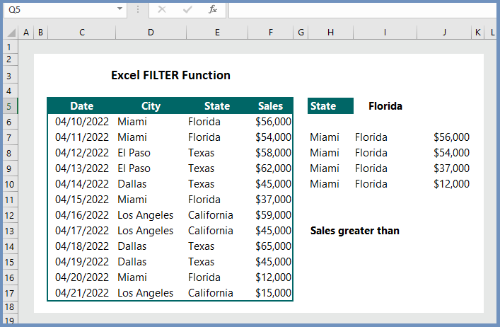
The FILTER Function we have used in the example above is already a dynamic one and we can easily extract data for other states by simply typing the name of the states or we create the data validation list for the names of the states. In our example, we have just changed the name of the state, and we can see that the data has been extracted.

4. #CALC! error and how to manage it:

If we supply any value that does not exist, Excel will return the #CALC! error. To manage this error type, we can tell Excel that we want “Not Found” message if wrong information is supplied. Let’s type Alaska in the cell I5 and see what happens. After typing ALASKA in the I5 cell, we are given a #CALC! error because the name Alaska does not exist in our data set.

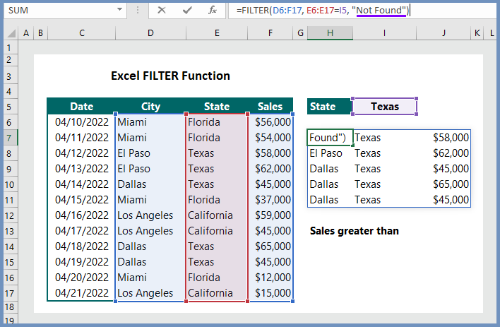
Suppose, we want the message “Not Found” instead of “#CALC! error. In that case, we need to add the last argument, and the formula would be =FILTER(D6:F17, E6:E17=I5, “Not Found“), which will return Not Found if we supply wrong information.

And after typing Alaska, we are given the following message:

5. How to FILTER values Greater than a certain value?

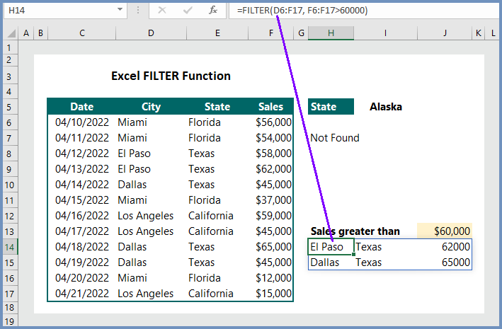
To extract values greater than a certain value, we need to use the math operators greater than (>). Let’s see how it works with our example.

Task: We want to see the city and states that have more than $60,000 sales revenue. The formula is

More readings:

MS Office Post

Excel AVERAGE Function